
What Exactly is a Convolution Anyway?
Introduction
I have a confession to make. I've never been very good at "black box programming". The reason for this is my insatiable curiosity. In learning to code I've rarely been satisfied with lessons and instructions that hand me some code and say here, since you're trying to do X use this. Not only do I need to know the solution but I need to understand why and how the solution works. And this mindset has saved me a lot of trouble many times. Although complete understanding of every line of code you use absolutely requires more time and effort up front, it saves much more time and effort downstream when you're trying to debug and troubleshoot issues. Many times I've seen naive programmers, when faced with a bug or issue, start arbitrarily changing lines of code without complete understanding hoping their changes will fix the issue. As often as not such an approach will add more complexity and potential for error to the solution even if it may initially seem to address the problem.
So I continue to maintain, when something you're trying to code doesn't behave as you expect, it pays to have a thorough and complete understanding of every line of code in your system. That's why, when I re-engaged neural network application development after many years of working on other things I wanted to revisit all the basics -- including the concept of convolution.
Convolution lies at the heart of much of what we see today in applied artificial intelligence. But what exactly is the convolution in convolutional neural networks and how does it work. For me, the best way to understand concepts -- especially mathematical concepts -- is to roll up my sleeves, get my hands dirty and interactively achieve understanding. I used to tell my students that in order to achieve deepest understanding you have to connect your input neurons to your output neurons. For me, especially when it comes to math, this means I have to do the exercises. I have to work with the formulas and equations rather than just read and memorize them. So this post is a result of such an exercise toward understanding. Yes, of course the convolution operation is already written into your machine learning libraries and frameworks. So, no, you don't have to worry about the math if you're really good at black-box programming. But if, like me, you crave a deep understanding of exactly what you're doing with your code, then it behooves you to do what it takes to deepen your understanding.
What is a Convolution?
Technically speaking, a convolution is a mathematical operation that can be applied to functions. The convolution operation is fundamental in many fields including signal processing, probability theory, and, by extension, machine learning.
Mathematically, the operation can be defined as the convolution integral; the product of two functions [denoted (f * g)(t)] where one function is reversed and shifted.
$$ (f \ast g)( t ) := \int_{-∞}^{\infty} f(x) g( t-x ) dx $$
Where:
-
f and g are the two functions undergoing convolution,
-
t is the independent variable of the convolution,
-
x is the integration variable, and
-
g(t-x) is the function, g, reversed and shifted by t units.
Understanding the Operation
Intuitively I find it useful to conceptualize convolution as a "sliding window". One function is reversed and shifted across the other with corresponding values multiplied and -- for discrete cases -- summed to generate the convolution at a given point.
Consider the following equation which expresses convolution as a discrete function:
$$ (a \ast b)[n] = \sum_{k=0}^{N-1} a[k] \cdot b[n-k] $$
For the discrete operation (which is what's actually applied in machine learning) we can achieve deeper understanding by working through through a simple example. Suppose we have two lists:
-
[1, 2, 3], and
-
[2, 3, 4]
Essentially, as defined above, convolving the lists simply means applying the operation to generate a new list given the two input lists. In other words we flip one operand and slide, or, shift it along the second to generate the output...
    1 2 3
4 3 2           1*2                2
    1 2 3
  4 3 2         1*3 + 2*2          7
    1 2 3
    4 3 2       1*4 + 2*3 + 3*2    16
    1 2 3
      4 3 2     2*4 + 3*3          17
    1 2 3
        4 3 2   3*4                12
So the result of the convolution for this simple example is [ 2, 7, 16, 17, 12 ]
To gain further insight into the operation (and practice with algorithms) you might consider implementing the algorithm in your favorite programming language. I've included my own naive python implementation as an appendix to this post. For further study you might even consider looking at the python numpy implementation, but you'll find that bit more complicated.
Applications
There are innumerable applications that rely on convolution. It is widely used in signal processing, probability theory, and image processing -- just to name a few broad fields -- and, of course, machine learning.
In machine learning, for purposes of image processing, the inputs to convolution (i.e., the source matrix and kernel) are 2D matrices. Again, toward deeper understanding of the mathematics, it's worth working through a few examples by hand.
Example
Let's consider the following matrix and associated kernel ( also referred to as filter ).
| $$ \begin{bmatrix} 1 & 2 & 0 & 3 \\ 4 & 1 & 0 & 2 \\ 3 & 2 & 1 & 0 \\ 0 & 1 & 2 & 4 \end{bmatrix} $$ | $$ \begin{bmatrix} 0 & 1 & 2 \\ 2 & 2 & 0 \\ 1 & 0 & 1 \end{bmatrix} $$ |
| Input Matrix: $M$ | Kernel: $K$ |
As we did for the simple one dimensional example above, we can obtain the convolution of the matrix and its kernel by sliding the kernel -- this time over the two dimensions. To keep things simple for this example, I'll consider just the positions where there is complete overlap between the kernel and its input (i.e., no padding). This case is technically referred to as a valid convolution. A valid convolution will yield a smaller matrix (fewer rows and columns) than the input. If we wanted an output matrix with the same dimensions (shape) as the input we'd have to "pad" the edges.
So, given $M$ and $K$ as defined above we want a valid convolution, $O$, of the two: $ O = M \ast K $ . What would that look like? Below I've illustrated the convolution steps highlighting the elements in $M$ contributing to the output at each step. The result of the convolution will be a 2 X 2 matrix.
| STEP 1 | STEP 2 | STEP 3 | STEP 4 |
| $$ \begin{bmatrix} \color{#08F} 1 & \color{#08F} 2 & \color{#08F} 0 & 3 \\ \color{#08F} 4 & \color{#08F} 1 & \color{#08F} 0 & 2 \\ \color{#08F} 3 & \color{#08F} 2 & \color{#08F} 1 & 0 \\ 0 & 1 & 2 & 4 \end{bmatrix} $$ | $$ \begin{bmatrix} 1 & \color{#08F} 2 & \color{#08F} 0 & \color{#08F} 3 \\ 4 & \color{#08F} 1 & \color{#08F} 0 & \color{#08F} 2 \\ 3 & \color{#08F} 2 & \color{#08F} 1 & \color{#08F} 0 \\ 0 & 1 & 2 & 4 \end{bmatrix} $$ | $$ \begin{bmatrix} 1 & 2 & 0 & 3 \\ \color{#08F} 4 & \color{#08F} 1 & \color{#08F} 0 & 2 \\ \color{#08F} 3 & \color{#08F} 2 & \color{#08F} 1 & 0 \\ \color{#08F} 0 & \color{#08F} 1 & \color{#08F} 2 & 4 \end{bmatrix} $$ | $$ \begin{bmatrix} 1 & 2 & 0 & 3 \\ 4 & \color{#08F} 1 & \color{#08F} 0 & \color{#08F} 2 \\ 3 & \color{#08F} 2 & \color{#08F} 1 & \color{#08F} 0 \\ 0 & \color{#08F} 1 & \color{#08F} 2 & \color{#08F} 4 \end{bmatrix} $$ |
| $\odot$ | $\odot$ | $\odot$ | $\odot$ |
| $$ \begin{bmatrix} 1 & 0 & 1 \\ 0 & 2 & 2\\ 2 & 1 & 0 \end{bmatrix} $$ | $$ \begin{bmatrix} 1 & 0 & 1 \\ 0 & 2 & 2\\ 2 & 1 & 0 \end{bmatrix} $$ | $$ \begin{bmatrix} 1 & 0 & 1 \\ 0 & 2 & 2\\ 2 & 1 & 0 \end{bmatrix} $$ | $$ \begin{bmatrix} 1 & 0 & 1 \\ 0 & 2 & 2\\ 2 & 1 & 0 \end{bmatrix} $$ |
Figure 1: Illustrates the convolution of the matrix, $M$, with the kernel, $K$. At each step, the elements of the kernel are multiplied against the elements of the input matrix (highlighted in blue).
In general, the equation for a 2D convolution can be expressed as follows:
$$ O(i, j) = \sum_{m=0}^{h-1} \sum_{n=0}^{w-1} I(i+m, j+n) \cdot K(h-1-m, w-1-n) $$
Where:
- $I(i+m, j+n)$ is the element of the input matrix at position $(i+m, j+n)$
- $K(h-1-m, w-1-n)$ is the corresponding element of the flipped kernel, and
- O(i, j) is the element of the output matrix at the position $(i, j)$.
All this means is simply that the output matrix $O$ is obtained by flipping the kernel and sliding it over the input, performing element-wise multiplication at each step along the way. The convolution at each position $(i,j)$ of the output matrix is simply the sum of the element-wise products at each step.
So for this example ...
Step 1. Flip the kernel by 180 degrees:
| $$ K_{180} = \begin{bmatrix} 1 & 0 & 1 \\ 0 & 2 & 2\\ 2 & 1 & 0 \end{bmatrix} $$ |
Step 2. Compute the matrix element value for each step in the convolution:
-
$O_{0,0} = (1\times1)+(0\times2)+(1\times0)+(0\times4)+(2\times1)+(2\times0)+(2\times3)+(1\times2)+(0\times1) = 11$
-
$O_{0,1} = (1\times2)+(0\times0)+(1\times3)+(0\times1)+(2\times0)+(2\times2)+(2\times2)+(1\times1)+(0\times0) = 14$
-
$O_{1,0} = (1\times4)+(0\times1)+(1\times0)+(0\times3)+(2\times2)+(2\times1)+(2\times0)+(1\times1)+(0\times2) = 11$
-
$O_{1,1} = (1\times1)+(0\times0)+(1\times2)+(0\times2)+(2\times1)+(2\times0)+(2\times1)+(1\times2)+(0\times4) = 9$
And so therefore the result of the convolution is the output matrix:
| $$ O = \begin{bmatrix} 11 & 14 \\ 11 & 9 \end{bmatrix} $$ |
And just to be sure, we can check the answer we obtained using python ...
import numpy as np
from scipy.signal import convolve2d
input = [
    [1, 2, 0, 3],
    [4, 1, 0, 2],
    [3, 2, 1, 0],
    [0, 1, 2, 4]
]

kernel = [
    [0, 1, 2],
    [2, 2, 0],
    [1, 0, 1]
]
output = convolve2d( input, kernel, mode='valid')
print ( output )
[[11 14]
 [11  9]]
Notice how we set the mode to valid. scipy uses padding by default for convolve2d.
So, the above example walks through the convolution of a 2d matrix and a kernel -- an operation commonly applied in image processing. Next let's consider application of convolutions to machine learning -- let's draw the connection to CNN's, or, convolutional neural networks.
Convolutional Neural Networks
So having done a bit of a deep dive into the mathematics of the convolution operation it's worth considering its application to machine learning. Again, convolution is ubiquitous in machine learning, but to launch into discussion here let's look at a very basic example from image processing.
Suppose we want a classification system that can learn to categorize images. Image classification systems are widely used -- consider for example medical imaging, object identification in satellite images, traffic control systems -- the possibilities are endless. But, again, at the heart of a wide range systems in use today lies the convolutional neural network, or, CNN.
The Models
To better understand CNN's and the impact of the application of convolutional layers I created two models in order to make some comparisons; a multi-layer peceptron and a convolutional variant of the model. A multi layer perceptron (MLP) is an artificial neural network that can be used to learn complex patterns in data. Here's some sample python code which defines an MLP using tensorflow:
# Define a simple Multi Layer Perceptron model
model_mlp = models.Sequential([
    layers.Dense(64*64, activation='relu', input_shape=(128 * 128,)),
    layers.Dense(4, activation='softmax')
])
If you aren't familiar with tensorflow don't sweat it. For now, the point is that this code defines a neural network with three layers; an input layer (which is capable of processing 128 X 128 pixel images), a hidden activation layer, and an output layer with 4 units (enabling classification into 4 categories).
MLP's can be enhanced through the addition of convolutional layers in the network architecture. Here's some code which enhances the basic MLP with a convolutional layer.
# Define a CNN model
model_cnn_4 = models.Sequential([
    layers.Conv2D(32, (3, 3), activation='relu', input_shape=(128, 128, 1)),
    layers.MaxPooling2D((2, 2)),
    layers.Flatten(),
    layers.Dense(128, activation='relu'),
    layers.Dense(4, activation='softmax')
])
The convolutional layer is defined with set of 32 3 X 3 filters. The filters are convolved across the input to generate feature maps. Randomly determined initially, the filter values are updated over the course of training (through backpropagation) -- enabling the system to settle into a state that optimizes classification for the training set. In other words, convolutional layers enable the system to extract features from the input which can enhance learning analogous to the ways in which we as humans perceive and learn!
Testing the Models
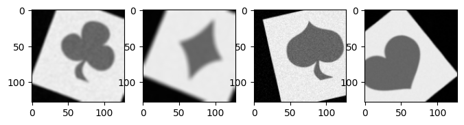
In order to test the models I created a data set based on four classes (drawn from the four suits represented in decks of playing cards).
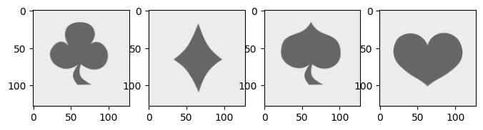
To create the data set I took the four exemplars (shown above) and applied basic data augmentation techniques. I introduced variability using geometric rotations and translations, adding varying degrees of blur, and injecting random noise. Here are four examples (one from each class) drawn from a set of 80 items generated to train the model.
The following graphs show the results of training and the training benefit obtained through convolution.
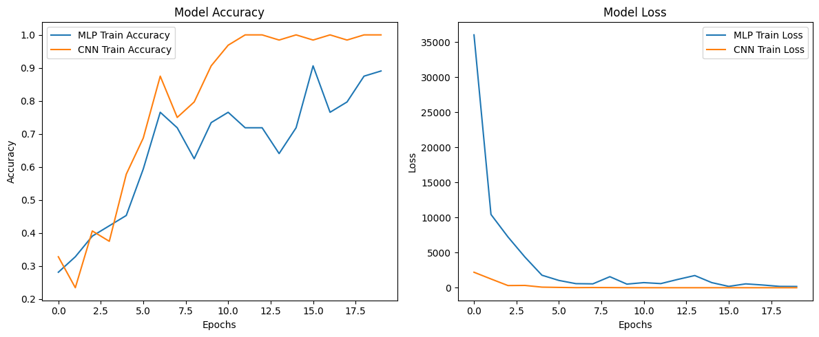
Figure 2: Model accuracy and loss obtained over twenty training epochs for the MLP and CNN models.
Figure 2 shows the training results obtained over 20 training epochs with the two models. The graphs represent model accuracy (left hand side) and loss (on the right). The model accuracy is a reflection of how accurate the model classification is across the data-set (i.e., the proportion of correct classifications). Loss is a representation of error. It's a measure of how far the model's predicted output deviates from the actual target output.
So what these learning curves show is how convolutional layers can enhance learning in neural networks. Both models learn the data set -- that is, both improve in accuracy over the course of training. But the convolutional model achieves much greater accuracy than the simpler MLP. Also, the convolutional layer allows the model to settle into an more optimal state more quickly as shown by the loss curves. So there you have it. The mechanics of the convolutional neural network.
Summary
In this blog post I've explored the mathematics of convolution in order to better understand it's application to machine learning. Starting with its definition as a continuous integral applied to two functions and considering its discrete counterpart I worked through a simple example in order to understand the mathematical concept. I then extended the discussion to consider convolution applied to 2D matrices (used ubiquitously in image processing). Finally, I provided a very simple comparison between a multi-layer perceptron model and one augmented with convolutional layers in order to see the benefit of using convolution to define CNN's. Hopefully, this post will help to deepen understanding of the building blocks of neural networks and encourage further exploration.
Appendix 1: My Naive Pass at Convolution -- An Exercise in Algorithm Implementation
This is just a naive python implementation -- an exercise solely intended to get those synapses firing. But, again, my philosophy is that in the same way doing push-ups enables you to exercise your muscles implementing algorithms enables you to exercise your brain.
def nn_convolve( a, b ) :
  '''
  My naive implementation of convolution ...
  '''
  b_flipped = np.flip( b )
  convolution = []
  start = len(b) - 1
  stop  = len(b)
  for i in range( len(a) + len(b) - 1 ) :
    k = 0
    j_range = range ( start, stop )
    for j in  j_range  :
      k += a[ i - (len(b)-1) + j ] * b_flipped[j]
    if start > 0 :
      start -= 1
    if i >= len( a )-1 :
      stop -= 1
    convolution.append(k)
  return np.array( convolution )
And some tests
a = np.array( [1, 2, 3] )
b = np.array( [2, 3, 4] )
print( nn_convolve ( a, b ) )
a3 = np.array( [1, 2, 3, 4, 1, 2, 3, 4] )
b2 = np.array( [0.1, 0.5] )
print( nn_convolve ( a3, b2 ) )
print( np.convolve ( a3, b2 ) )
The key highlights regarding the solution are that it (1) flips the kernel and then computes the sum of element-wise multiplications as you slide the kernel across the signal (again, the essence of convolution).
Appendix 2: Exploring the numpy Implementation
For the truly intrepid, it may well be worth studying the python numpy implementation of the convolve function. The implementation is quite a bit more complex than our naive version, because (1) it is optimized for large arrays by using FFT to calculate the convolution, and (2) it is implemented in C for performance. At the time of this writing I determined that the implementation uses a python wrapper (numeric.py) and calls low-level C++ functions in the multi-array module as illustrated in the following diagram.

Figure 3: High level architecture of the numpy convolution implementation. Essentially, the 'convolve' function defined in numeric.py calls a low-level C implementation defined in multiarraymodule.c. Note: if you want to click directly into the source code try opening the diagram in a new tab. You should then be able to click the links...
The heart of the algorithm's implementation lies in _pyarray_correlate since convolution is mathematically equivalent to cross-correlation (except for the reversal of the filter/kernel). Additional functionality (e.g., determining whether FFT optimization is warranted, flipping the kernel, checking for error conditions on function arguments) are added for convolution.